-
Linear models include:
-
| AR |
Autoregressive errors |
| ARCH |
Autoregressive conditional
heteroscedastic errors |
| OLS |
Ordinary least squares |
| PLS |
Partial least squares |
| POISSON |
Poisson regression |
| QR |
Quantal response (logit, probit,
ordered) |
| STEPWISE |
Stepwise regression |
| SURE |
Seemingly unrelated regression
estimation |
| VAR |
Vector autoregressive |
| 2SLS |
Two stage least squares |
| 3SLS |
Three stage least squares |
- Descriptive statistics, elasticities,
automatic treatment of missing values, weighted analysis
and White or Newey-West robust standard errors are
standard. Lag specification such as y(-1) is
supported, as are PDL structures. Diagnostics for single
equations include Godfrey's test for residual serial
correlation, Ramsey's RESET test for functional form, Jarque-Bera's
test for normality of residuals, Breusch-Pagan test for
heteroscedasticity, and Chow's test for stability.
-
Non-linear models include:
| FIML |
Full information maximum likelihood |
| GMM |
Generalized method of moments |
| ML |
Maximum likelihood |
| NLS |
Non linear least squares |
Step-algorithms include:
| BFGS |
Broyden-Fletcher- Goldfarb-Shanno
algorithm |
| BHHH |
Berndt-Hall-Hall- Hausman algorithm |
| DFP |
Davidon-Fletche-Powell algorithm |
| DW |
Dennis-Wolkowicz algorithm |
| GA |
Genetic algorithm |
| GAUSS |
Linearized in variables algorithm |
| GN |
Gauss Newton algorithm |
| GO |
Global optimization |
| NM |
Nelder-Meade search algorithm |
| NM |
Newton-Raphson algorithm |
| SA |
Simulated annealing |
Step-size methods include:
| LS |
Line search |
| QP |
Quadratic programming |
TRUST
|
Trust region |
Both the White
and Newey-West robust estimators are supported, as well as the Murphy-Topel
two step estimation. The
defaults used during non-linear estimation can be altered
heuristically during execution, or through a script file.
Gradients, Hessian, and Jacobian are estimated
numerically as the default; however they can be written
as a procedure by the user.
Coefficient restrictions can be imposed with
PARAM, and investigated using ANALYZ,
which can be used following either
linear or non-linear estimation. Descriptive statistics,
automatic treatment of missing values, and weighted
analysis are standard.
The maximum likelihood (ML)
procedure permits the estimation of any specified
likelihood - Gaussx includes examples for a number of non-linear
processes:
| AGARCH |
Asymmetric GARCH process |
| ANN |
Artificial neural network |
| ARCH |
Autoregressive conditional
heteroscedastic process |
| ARFIMA |
Autoregressive fractional integrated
moving average process |
| ARIMA |
Autoregressive integrated moving average
process |
| ARMA |
Autoregressive moving average process |
| DBDC |
Double-bounded dichotomous choice
process |
| EGARCH |
Exponential GARCH process |
| FIGARCH |
Fractionally integrated GARCH
process |
| FMNP |
Feasible multinomial probit |
| FPF |
Frontier production function process |
| GARCH |
GARCH process |
| IGARCH |
Integrated GARCH process |
| KALMAN |
Kalman filter |
| LOGIT |
Binomial logit process |
| MGARCH |
Multivariate GARCH process |
| MNL |
Multinomial logit |
| MNP |
Multinomial probit |
| MSM |
Markov switching models |
| MVN |
Multivariate normal process |
| NEGBIN |
Negative binomial process |
| NPE |
Non parametric estimate |
| ORDLGT |
Ordered logit process |
| ORDPRBT |
Ordered probit process |
| PGARCH |
Power GARCH process |
| POISSON |
Poisson process |
| PROBIT |
Binomial multivariate probit process |
| SV |
Stochastic volatility process |
| TGARCH |
Truncated GARCH process |
| TOBIT |
Tobit process |
| VARMA |
Vector autoregressive moving average
process |
| WHITTLE |
Local Whittle process |
- Constrained optimization is
supported under FIML,
GMM, ML, NLS and RSM.
The parameter constraints can be linear or non-linear.
The estimation is undertaken using sequential quadratic
programming. The constrained confidence region for any
specified confidence level for each parameter is
calculated.
-
-
A choice of numeric, analytic, or symbolic derivatives is available for FIML,
ML and NLS.
The default method of deriving gradients and Hessians is numeric, using finite
differencing. Analytic derivatives are specified by the user, while symbolic
derivatives are calculated using the automatic differentiation capability of
Maple 9. Symbolic gradients and Hessians can be saved as procedures and
reused. Analytic differentiation work only for Gaussx for
Windows, and requires Maple 9 or higher.
-
- A complete range of time series
analysis is available under Gaussx, including ARMA,
ARIMA and ARFIMA for single equations,
and VAR and VARMA
for multiple equations. ARIMA
includes full identification, estimation
and forecasting with graphical presentation. Systems of
transfer functions can be specified, with a separate
moving average structure for each equation. Markov switching models (MSM)
include AR components and non-linear state equations. Spectral
analysis is also supported
-
- Linear LDV models
include binomial probit, multinomial logit, and ordered
logit and probit; in each case the marginal effects and
elasticities, and their variances, evaluated at the mean,
are available. Diagnostics include Pearson Residual test, Deviance test,
Bera, Jarque and Lee normality test (probit), Hosmer-Lemeshow test,
as well as concordance/discordance measures. For both probit and logit, Mills ratio is
available allowing correction for selection bias.
Heckman's two step procedure (HECKIT)
incorporates Greene's covariance correction. Non linear
multinomial logit and probit
(MNL and MNP) are available using ML; for the latter, high dimensional
integration is carried out either exactly using the GAUSS
CDFMVN
function, or through simulation using
the smooth recursive simulator. Double-bounded (DBDC)
models are also supported. For models with large number of
alternatives, feasible multinomial probit (FMNP), which does not require
parameterization of the covariance matrix, is available for both ranked
and non-ranked data.
PANEL estimates the coefficients of a linear regression model for panel data.. Both fixed effects and random effects (error components model) for balanced and unbalanced models are supported. The Hausman test for testing the orthogonality of the random effects and the
regressors, and the Bresuch Pagan test for random effects are implemented.
-
- A variety of Arch and Garch models are supported; these include linear ARCH,
single equation non-linear ARCH, AGARCH, EGARCH, FIGARCH, GARCH, IGARCH, PGARCH and TGARCH. Residuals can be distributed
normal, Student-t, or GED. Garch in the mean, leverage
options, and MA residuals are all supported. Stability
and positive variance is secured using the constrained
optimization facilities.
-
- Multivariate GARCH (MGARCH) estimated over a system of equations,
with the option of weakly exogenous variables, is also
supported, under both the VEC and BEKK
formulation. MGARCH-M is also available.
-
Survival models (life data regression) are estimated using ML for both
uncensored or censored data. Supported parametric models include:
| BETA |
Beta process |
| COX |
Cox proportional hazards process |
| EXPON |
Exponential process |
| GAMMA |
Gamma process |
| GOMPERTZ |
Gompertz process |
| GUMBEL |
Gumbel (largest extreme
value) process |
| INVGAUSS |
Inverse Gaussian process |
| LOGISTIC |
Logistic process |
| LOGLOG |
Loglogistice process |
| LOGNORM |
Log normal process |
| NORMAL |
Normal process |
| PARETO |
Pareto process |
| PEARSON |
Pearson process |
| SEV |
Smallest extreme value process |
| WEIBULL |
Weibull process |
Survival measures, based on the last survival
model estimation, include survival rate, inverse survival
rate, hazard rate, cumulative hazard rate and cumulative failure rate. For each measure, the rate, the standard error, and the lower and upper confidence band
are reported for each observation. Residuals include ordinary,
standardized, Cox-Snell, deviance, martingale, Schoenfeld, scaled Schoenfeld
and score. The indices can be linear or non-linear.
The Cox proportional
hazards model supports the same survival and residual measures; ties are
treated using the Breslow, Efron, discrete and exact methods.
Non-parametric
processes (support the same survival measures, using either the Kaplan-Meier or Nelson-Aalan algorithms.
-
- Methods include single, double,
Holt-Winters, and seasonally additive or multiplicative
Holt-Winters. Smoothing parameters can be user specified
or optimally estimated by Gaussx.
-
- Denosing of signals and time series is accomplished using wavelet
shrinkage methods. Thresholds include universal, minimax and SURE.
-
-
- Non-parametric and semiparametric
analysis under Gaussx permits the estimation of
the window width and the weights in the semiparametric
index using cross validation under maximum likelihood.
For the single index case, the FFT is used
to speed calculation. Conditional response coefficients
are determined for the density, conditional mean,
discrete and smeared case.
-
- The hidden and output weights in a
feed forward network with a single hidden layer are
estimated using non-linear optimization, rather than back
propagation. Transfer functions include Arctan, Gaussian,
Halfsine, Linear, Sigmoid, Step, and Tanh. Output
processing includes levels, density, and maximum.
-
- Analysis with the Kalman Filter
allows for the estimation of state vectors, with smoothing, time varying transition matrices (ie. each
element is a function), and the estimation of the
elements of the Kalman matrices using ML. Stochastic
Volatility models (SV) are estimated using quasi ML based on a Kalman Filter
model.
-
- Robust estimation (ROBUST) of linear models when the distribution
of the residual is unknown is undertaken using Quantile Regression
(interior point algorithm), as well as using reiterated weighted least
squares for Least Absolute Deviation, Huber's t
Function, Ramsay's E Function, Andrew's Wave
Function, and Tukey's Biweight. The parameter covariance matrix is
estimated using bootstrapping.
-
- Static and dynamic forecast values
and residuals are available for all estimations. Systems
of non-linear equations can be solved statically or
dynamically. An impulse response function is available
for VAR models. OLS forecasts also
include prediction error, bounds, studentized residuals,
Cook's D, HAT, DFFITS and DFBETAS.
ML
forecasts include log likelihood, GARCH forecasts include conditional
variance, QR forecasts include probabilities
and category, and ARFIMA forecasts include
both naive and best linear predictor. After an estimation, FORCST
can evaluate the predicted value and standard errors for variables that are non-linear functions of
estimated parameters.
-
- Monte-Carlo simulation (MCS) can be
carried out over a block of code, using both bootstrap
and jackknife methods. Output for the selected variables
is shown dynamically on the screen, and final output
includes cumulants and quantiles. Latin Hypercube Sampling (LHS)
is provided as an alternative to MCS, and
allows for nearly orthogonal and correlated sampling.h
-
- For Bayesian analysis, Markev Chain Monte Carlo (MCMC)
is carried out over user supplied distributions and priors. Diagnostics
include Geweke numerical standard error, relative numerical efficiency and
a Chissq test for stability. Examples
include:
| AR(k) with hetersoscedastic residuals |
| Binomial probit |
| Heteroscedastic binomial probit |
| Multinomial probit |
| OLS, residuals distributed normal |
| OLS, residuals distributed t |
| OLS, heteroscedastic residuals |
| Poisson |
| Tobit |
| SURE |
-
- STATLIB consists of a set of procs for evaluating
density functions, which can be used from GAUSS
or Gaussx; these provide the
PDF, the CDF,
the inverse CDF and random sampling from
over 60 distributions.
Continuous Distributions
| beta |
beta4 |
boxcox |
burr |
| cauchy |
chisq |
chisq_scaled |
erf |
| expon |
f |
f_scaled |
fatiguelife |
| fisk |
foldednormal |
frechet |
gamma |
| ged |
gengamma |
genlogistic |
genpareto |
| gumbel |
halfnormal |
invgamma |
invgauss |
| johnson_sb |
johnson_sl |
johnson_su |
laplace |
| levy |
loggamma |
logistic |
loglog |
| lognorm |
maxwell |
ncchisq |
ncf |
| nct |
normal |
pareto |
pearson |
| pert |
power |
rayleigh |
reciprocal |
| sev |
skewnormal |
students_t |
t_scaled |
| triangular |
uniform |
vonmises |
weibull |
-
Discrete Distributions
| bernoulli |
binomial |
geometric |
hypergeom |
| logarithmic |
negbin |
poisson |
rectangular |
| step |
|
|
|
-
Sampling from a truncated multivariate normal, multivariate t, and
Wishart distribution, sampling from a specified cdf, correlated
sampling using COPULA and multivariate random sampling (MVRND),
as well as sampling with and without
replacement are also available.
-
-
- Bitwise AND, EQV, OR XOR, NOT, and
SHFT are supported, as are conversions from decimal to base, and
base to decimal. Quasi random variables (Sobol) are also supported.
-
- Tools include:
-
| AMORT |
Amortization schedule |
| FRONTIER |
Markowitz efficient frontier |
| FV |
Future value |
| GINI |
Gini coefficients |
| LP |
Linear programming |
| MCALC |
Mortgage calculation |
| ME |
Maximum entropy |
| PV |
Present value |
| RSM |
Response surface methodology and
multi response optimization |
| SOLVE |
Solve a system of equations |
| SPECTRAL |
Power spectrum estimation |
| WELFARE |
Consumer surplus (CV, EV, MS and
deadweight loss) |
-
- The TEST command includes both parametric
and nonparametric tests:
-
| Parametric |
|
|
|
AD |
Anderson-Darling normality test,
with censoring |
|
ANOVA |
Analysis of Variance |
|
ARCH |
Engle's ARCH test. |
|
BARTLETT |
Bartlett's Test for equality of variances: |
|
BKW |
Belsley-Kuh-Walsh collinearity test |
|
BP |
Breusch Pagan homoscedasticity
test |
|
CHISQ |
Chi squared test. |
|
CHOW |
Chow stability test. |
|
DF |
Dickey-Fuller unit root test. |
|
EG |
Engle-Granger cointegration test |
|
F |
F test |
|
FTEST |
Linear restriction test |
|
GRANGER |
Granger causality test |
|
HANSEN |
Hansen test of overidentifying
restrictions. |
|
HAUSMAN |
Hausman specification test |
|
JB |
Jarque-Bera normality test. |
|
JTEST |
Davidson and MacKinnon's J-Test for
non-nested estimations. |
|
KPSS |
KPSS stationarity test. |
|
LBQ |
Ljung-Box Q test. |
|
LM |
Lagrange
Multiplier test |
|
LRT |
Likelihood ratio test |
|
NW |
Newey West D test |
|
PIT |
Probability integral transformation
test |
|
PPC |
Probability plot correlation test |
|
RECURS |
CUSUM and CUSUM-squared
tests for stability |
|
SF |
Shapiro-Francia normality test,
with censoring |
|
SW |
Shapiro-Wilks normality test, with
censoring |
|
THEIL |
Thiel's decomposition
of two vectors |
|
TTEST |
T test |
|
WALD |
Wald test |
|
WELCH |
Welch's test for equality of means |
|
|
|
| Non-Parametric |
|
|
|
BF |
Brown-Forsythe test of scale |
|
CONOVER |
Conover test for treatment |
|
FRIEDMAN |
Friedman test for treatment |
|
KS |
Kolmogorov-Smirnov test |
|
KURTOSIS |
Kurtosis test |
|
KW |
Kruskal-Wallis test of location |
|
LEVENE |
Levene test of scale |
|
MOOD |
Mood's test of location |
|
MW |
Mann Whitney U test of location |
|
OBRIEN |
O'Briens test of scale |
|
RUNS |
Runs test of randomness |
|
SIGN |
Sign test for treatment |
|
SKEWNESS |
Skewness test |
|
WALSH |
Walsh test for treatment |
|
WILCOXON |
Wilcoxon test for treatment |
-
- Memory allocation and all file
control is handled automatically. Data size for non-AR
estimation is limited by disk capacity only. External
data can be imported as delineated ASCII,
packed ASCII, binary, Lotus, Excel,
GAUSS data
files, GAUSS format files, and Gaussx save
files. Data can be exported as ASCII, binary, Gaussx or GAUSS
data files. Under Windows, import/export
is available for Lotus, Excel, Quattro, Dbase, Symphony,
Paradox, Foxpro, Clipper and both delineated and packed ASCII. Variables in a
Gaussx dataset can be user selected with the KEEP
or DROP commands.
-
- Data transformation (GENR, FEVAL)
permits the use of all GAUSS operations and all the
GAUSS functions, such as
FFT,
all GAUSS distributions, random number generators,
etc. Thus all the power of GAUSS is
available in Gaussx. However sample selection (SMPL)
makes coding far simpler, and data input/output is
transparent. Stochastic data can be created using 15 distributions with DGP,
and data can be filtered with 7 types of FILTER. Other
tools include vector convolution and deconvolution, difference and inverse
difference, and vector interpolation.
-
- A number of descriptive measures are provided:
-
| ANOVA |
N-way analysis of variance for fixed, random or mixed
models. Nested and interaction effects, variance components. |
| CATALOG |
Descriptive comment for each variable |
| CLUSTER |
Cluster groups and dendrogram |
| CORDIM |
Correlation dimension |
| COVA |
Means, standard deviations, minimum
and maximum, sum, covariance and correlation matrices,
autocorrelogram, partial autocorrelogram. |
| CROSSTAB |
Cross tabulation of data |
| DIVISIA |
Divisia indices |
| FREQ |
Frequency distributions |
| LYAPUNOV |
Lyapunov exponent |
| PRIN |
Principal components |
| SAMA |
Seasonal adjustment (including Census X12), |
| SVD |
Singular value decomposition |
| TABULATE |
Tabulates data across two class variables |
-
-
- Cluster analysis creates an hierarchical cluster tree of
the data, and optionally graphs the tree - a
dendrogram. Five distance metrics and four linkage methods are available.
-
-
- Graphical output (PLOT, GRAPH, COVA) is available using either Publication Quality
Graphics or, if installed, GAUSSPlot. Line and scatter graphs/plots are supported.
Gaussx has
full support for all GAUSS PQG routines, while for
GAUSSPlot,
interactive customization of a graph can be saved and used in subsequent
sessions.
-
- All GAUSS commands, logical goto, DO loops,
and GAUSS procs can be used within a Gaussx file. In addition,
Gaussx provides a number of programming commands; these include
macro definitions for formulae, LOOP control
for multisectored data, GROUP
control (like BY in SAS) and recursive
LIST names. A timer
control is available to simulate realtime analysis.
-
- Symbolic algebra can be used for
symbolic differentiation and integration, exact linear
algebra, and equation solving. Gaussx uses
Maple and/or Mathematica to permit GAUSS
to
undertake symbolic manipulation. Simply include the
Maple/Mathematica statements within the command file,
select the statements, and click the Maple or Mathematica
button. This works only for Gaussx for
Windows, and requires Maple, rev 4 or higher or
Mathematica, rev 3 or higher.
-
- A number of mathematical tools to augment GAUSS
-
| ACF |
Autocorrelation function |
| ACV |
Autocovariance function |
| COMBS |
All k combinations of a vector |
| DECONV |
Deconvolution |
| INTERP |
Interpolation |
| INVERT |
Find the inverse values of a function. |
| ISCHAR |
Tests for a character vector |
| PERMS |
All permutations of a vector |
| POLYDIV |
Polynomial division |
| POLYINV |
Polynomial inversion |
-
-
- GAUSS statements can be included within the
command file. Gaussx variables can be made global
(FETCH), and
global variables can be stored in the Gaussx workspace (STORE).
Thus maximum flexibility is achieved by being able to mix GAUSS
and
Gaussx commands. User written procs can be included within Gaussx formula definitions. In addition, most
GAUSS application modules can be run directly
from a Gaussx file.
-
- The complete source code, written
in GAUSS, is included. Thus even if you don't
want all the features of Gaussx, you
can extract a particular procedure and use it in your own GAUSS
programs -- procedures such as inverse
cumulative normal density function, Gibbs sampling,
smooth recursive simulator (GHK),
multivariate normal rectangle probabilities for any
dimension, random sampling from a multivariate truncated
distribution, maximum entropy estimation, quasi random
sequences, bitwise arithmetic and more. And because of
its modular design, you can also add your own procedures
to Gaussx, or modify any Gaussx procedure to fit your requirements.
-
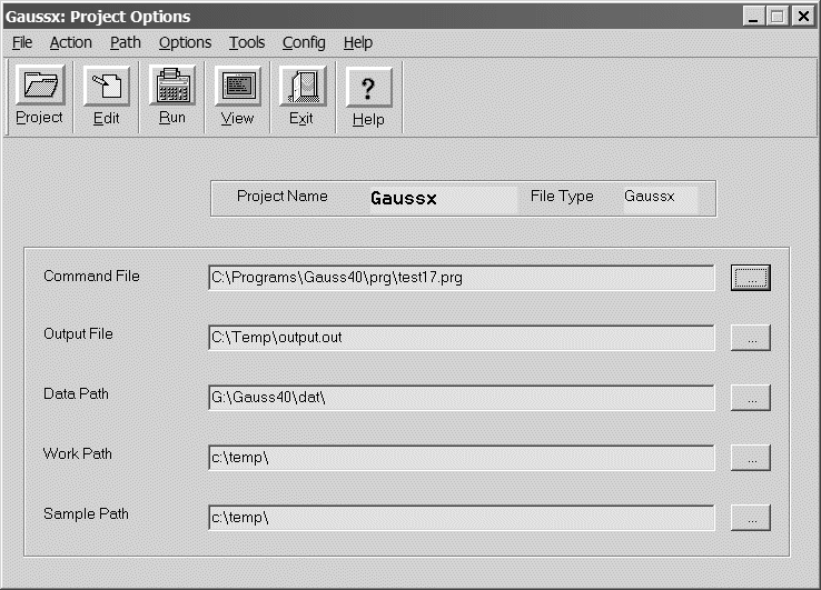
| Windows Project Control Screen |
- Project
management is provided for Gaussx for Windows, with up to 100 separate
applications, each associated with different file names
and paths. Gaussx is network compatible - thus on a
network, each client has its own project and
configuration file. Project management can also be used to manage pure
Gauss applications.
-
- During execution of a command file,
pop-up help is available to explain the current screen,
using Alt-H. Under Windows, context sensitive help
(F1) is available to provide
the complete syntax of each Gaussx command.
-
- Gaussx can be run on a single machine or on a
network, under either Windows, Unix or Mac.
GAUSSX for
WINDOWS runs under
Windows 2000, XP, Vista, Win7 and Win8. Gaussx for Windows requires
GAUSS for Windows 6.0 or higher, and about
7 MB of hard drive. GAUSSX
supports both 32 bit and 64 bit versions of GAUSS.
GAUSSX
for UNIX and MAC runs in Terminal mode. Networking is built in, so
that individuals will each have their own configuration file.
The econometric specifications for the Unix version is
identical to the Windows version.
Gaussx for Unix has been designed to be machine independent by writing the
entire package in GAUSS. Thus, if your Unix machine
runs GAUSS, it will run Gaussx. Gaussx requires
Gauss for Unix 4 or higher, and about 1MB of hard
drive.
The package includes: source code,
menu driven installation, tutorial, 50 sample command
files with index, compiled HTML help for syntax, and a complete 450 page manual
in PDF format (with
reference section and index). A hard copy version of the manual is
an optional extra. Single-user, network and
student versions are available. Academic prices start at
about $225,
with a 30 day, no-question refund policy, and free
technical support by phone and the internet. For
technical information, contact Econotron Software, and for ordering information, contact
Aptech Systems.